
Approximate Solutions for Navier-Stokes
Enroll to start learning
You’ve not yet enrolled in this course. Please enroll for free to listen to audio lessons, classroom podcasts and take practice test.
Interactive Audio Lesson
Listen to a student-teacher conversation explaining the topic in a relatable way.
Introduction to Navier-Stokes Equations
🔒 Unlock Audio Lesson
Sign up and enroll to listen to this audio lesson

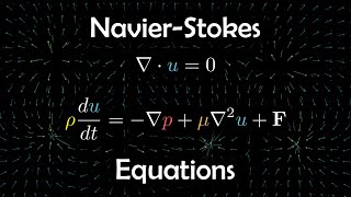
Today, we're diving into the Navier-Stokes equations, which are foundational in describing fluid motion. These equations enable us to analyze various flow conditions, such as those around solid boundaries and moving objects.

How do we apply these equations to different scenarios, like flow past a building?
Great question! Essentially, we apply the Euler equations to describe flow around structures when the flow is considered incompressible and non-viscous. The equations help predict flow patterns, including any regions affected by turbulence.

But what happens when we have turbulence?
When turbulence is present, the Navier-Stokes equations provide complexity due to non-linear terms, and that's where approximations become helpful.
In summary, Euler equations represent ideal flows, whereas Navier-Stokes accommodate viscous flows.
Velocity Potential Functions
🔒 Unlock Audio Lesson
Sign up and enroll to listen to this audio lesson

Next, let's discuss velocity potentials. They allow us to reduce the complexity of fluid motion analyses. Instead of working with three velocity components, we can express them with a single scalar potential function, phi.

What are the conditions for using a velocity potential?
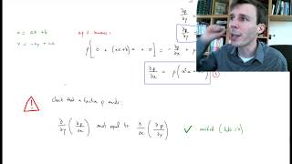
Excellent point! These functions are valid under irrotational flow conditions, meaning the fluid exhibits negligible rotational characteristics.

Could you show us how to derive those components from phi?
Certainly! The velocity components can be expressed as derivatives of phi, namely, u = ∂φ/∂x, v = ∂φ/∂y, and w = ∂φ/∂z. This simplifies multiple equations into one.
To wrap up, velocity potentials represent a powerful analytical tool when dealing with incompressible flows.
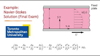
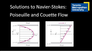
Flow Between Fixed and Moving Plates
🔒 Unlock Audio Lesson
Sign up and enroll to listen to this audio lesson
Now, let's bring our focus to flow between fixed and moving plates. This is a classic example of how we solve for viscous flow using Navier-Stokes equations.
What assumptions do we need to make for this case?
We assume steady, fully developed flow along with negligible gravity effects for horizontal plates. This dramatically simplifies the equations.
How does that change our approach?
We simplify the Navier-Stokes to ordinary differential equations, allowing us to integrate and find velocity profiles easily.
For instance, in a linear flow case, the velocity distribution will be linear due to shear between plates.
In conclusion, understanding these assumptions significantly reduces complexity when working with the Navier-Stokes equations.
Calculating Pressure Gradients
🔒 Unlock Audio Lesson
Sign up and enroll to listen to this audio lesson
Finally, we will discuss pressure gradients in flowing fluids, particularly in the frame of two fixed plates.
Why is it important to consider pressure in our flow calculations?
Understanding pressure gradients is crucial because they drive fluid movement in viscous flows. The gradient will dictate the velocity profile we observe in the flow.
How do we calculate that in practice?
We apply the Navier-Stokes and continuity equations to derive our functions explicitly. Integration helps us find pressure distribution across the flow area.
To summarize, pressure gradients are at the heart of understanding dynamic fluid behavior and allow us to predict how fluids will behave under various conditions.
Introduction & Overview
Read summaries of the section's main ideas at different levels of detail.
Quick Overview
Standard
The section provides an overview of how to derive useful approximations from the Navier-Stokes equations applicable to simple flow problems involving incompressible viscous fluids. Key concepts discussed include velocity potentials, conditions for irrotational flow, and methods for solving for velocity distributions in various flow scenarios. Practical examples and exercises illustrate the importance and application of these concepts in fluid mechanics.
Detailed
Approximate Solutions for Navier-Stokes
This section delves into the intricacies of the Navier-Stokes equations and how they can be simplified to obtain solutions that are applicable to various fluid mechanics problems. Initially, the instructor revisits Bernoulli's equations and their derivation from the Navier-Stokes equations, outlining the significance of velocity potentials in fluid flow. The focus then shifts to exploring viscous flow between fixed and moving plates, emphasizing the scenarios of parallel plates undergoing shear deformation due to flow.
Key Concepts Covered:
- Euler Equations: The section begins with a brief explanation of Euler equations as applied to incompressible and non-viscous flows, especially around objects like high-rise buildings. The limitations of these equations near turbulent flow regions are highlighted.
- Velocity Potentials: The teacher introduces the concept of velocity potential functions as alternatives to multiple velocity components (u, v, w), simplifying the analysis. They are derived as gradients of a scalar function phi, applicable under irrotational flow conditions. The significance of this transformation is underscored, alongside its associated conditions.
- Flow between Plates: The discussion progresses to the mathematical formulation for incompressible viscous flow between two plates, one fixed and the other moving. Key assumptions such as neglecting gravity in horizontal flows and establishing fully developed flow conditions are made. The discussion of Navier-Stokes equations simplifies the complexity of fluid flow to achieve ordinary differential equations that facilitate analytical solutions.
- Pressure Gradients and Shear Stress: The section also elaborates on cases where flow occurs due to pressure gradients, particularly in scenarios involving two fixed plates. The shear stresses at the plates are calculated using the derived velocity profiles.
This section establishes foundational knowledge critical for both theoretical understanding and practical applications within the realm of fluid mechanics, paving the way for further exploration into boundary layer theory.
Youtube Videos

Audio Book
Dive deep into the subject with an immersive audiobook experience.
Introduction to Approximate Solutions
Chapter 1 of 7
🔒 Unlock Audio Chapter
Sign up and enroll to access the full audio experience
Chapter Content
Good morning all of you. Today we are going to discuss on nebustic locations and its approximation for simple flow problems.
Detailed Explanation
In this section, we introduce the idea of approximate solutions to the Navier-Stokes equations, which are fundamental in fluid mechanics. The professor starts by engaging students in the discussion about how to derive simpler forms of these equations to address specific flow scenarios. The emphasis is on the practicality of these approximations for real-world problems, which often involve complex flow patterns.
Examples & Analogies
Think of it like using a shortcut when driving. When you are in a hurry, you might take a route that is not the most direct but helps you reach your destination more quickly. In fluid mechanics, using approximate solutions allows engineers to simplify complex equations so they can analyze fluid flows faster and more effectively.
Recap of Bernoulli's Equation
Chapter 2 of 7
🔒 Unlock Audio Chapter
Sign up and enroll to access the full audio experience
Chapter Content
As we discussed in the last class how we can derive the basic Bernoulli's equations from Navier-Stokes equations.
Detailed Explanation
This chunk revisits the derivation of Bernoulli's equation from the Navier-Stokes equations. Bernoulli's equation provides a relationship between the pressure, velocity, and elevation in a flowing fluid. By recalling how Bernoulli's equation can be simplified from the more complex Navier-Stokes equations, students see the utility of approximations in fluid mechanics. This background knowledge is essential before moving into more detailed approximations.
Examples & Analogies
Imagine you are at a water park. When you go down a water slide, you feel a rush of speed, but at the bottom, there's a calm pool waiting for you. This experience metaphorically reflects how energy changes within a fluid flow: the fluid may have high speed (kinetic energy) at certain points and high pressure (potential energy) at others, similar to how Bernoulli's equation balances these aspects.
Velocity Potentials and Flow Fields
Chapter 3 of 7
🔒 Unlock Audio Chapter
Sign up and enroll to access the full audio experience
Chapter Content
Before going that let me I just write down the basics equations is the Euler equations.
Detailed Explanation
Here, the discussion shifts to velocity potentials and their importance in analyzing fluid flow. Velocity potentials simplify the analysis by allowing us to represent the velocity field with a single scalar function rather than multiple vector components. This aspect is crucial because it shows the connection between scalar potentials and the behavior of fluid flows, especially in conditions where the flow is irrotational.
Examples & Analogies
Picture a large lake. The movement of water at the surface can often be caused by a flow of wind, making the surface appear active and complex. However, if we consider the movement of the water as a larger wave pattern, we could use a single potential function to describe it instead of considering every little ripple individually. This is similar to how velocity potentials can simplify the understanding of fluid flows.
Conditions for Irrotational Flow
Chapter 4 of 7
🔒 Unlock Audio Chapter
Sign up and enroll to access the full audio experience
Chapter Content
Thus if I define it the velocity is a gradient of phi, phi is a velocity potential function at which condition thus this is what justified it.
Detailed Explanation
In this segment, the conditions necessary for the use of velocity potentials are explained. Specifically, it indicates that for the velocity potentials to apply, the flow must be irrotational. An irrotational flow implies that the fluid elements are not rotating about their own axes, which is a key characteristic that allows the velocity field to be described as the gradient of a scalar potential function.
Examples & Analogies
Think of a calm, perfectly still water surface. The lack of disturbances means there’s no rotational movement in the water — it’s irrotational. Similarly, when analyzing certain flows in fluid mechanics, knowing that the flow behaves nicely (irrotational) allows us to use simpler mathematical tools to describe the flow.
Visualizing Flow with Stream Functions
Chapter 5 of 7
🔒 Unlock Audio Chapter
Sign up and enroll to access the full audio experience
Chapter Content
So we need to draw the streamlines and the potential lines to show it that because just you interpreted the gradient of the velocity potential functions indicates as the velocity field.
Detailed Explanation
This point emphasizes the importance of visualizing flow fields using streamlines and potential lines. Streamlines are lines that indicate the path followed by fluid particles, while equipotential lines represent surfaces with the same potential. Understanding these graphical representations helps to analyze the behavior of fluid flow around different structures more intuitively.
Examples & Analogies
Imagine a flowing river. The paths that leaves create on the surface of the water as they drift downstream represent streamlines — they visualize how particles are moving with the current. Using these visualizations, an engineer can better predict how structures like bridges might affect water flow, much like we analyze fluid movements.
Applications of Velocity Potential and Stream Functions
Chapter 6 of 7
🔒 Unlock Audio Chapter
Sign up and enroll to access the full audio experience
Chapter Content
Even if you solve the problems using computational fluid dynamics tools but always you can draw the streamlines you can draw the equipotential lines then you try to understand it.
Detailed Explanation
This chunk discusses the continuous relevance of drawing streamlines and equipotential lines even when modern tools such as Computational Fluid Dynamics (CFD) are utilized. The ability to visualize flow patterns can greatly aid in interpreting results from CFD simulations, allowing engineers to relate their computational findings back to physical phenomena.
Examples & Analogies
Think of using a GPS to find your way. While the GPS gives you detailed instructions, visually knowing the layout of the area aids your understanding and helps avoid getting lost. Similarly, plotting streamlines and potential lines enhances the comprehension of flow dynamics, ensuring that engineers correctly interpret CFD outputs.
Navier-Stokes Equation Approximations
Chapter 7 of 7
🔒 Unlock Audio Chapter
Sign up and enroll to access the full audio experience
Chapter Content
Now coming back to doing some simple approximations using Navier-Stokes equations to get simple solutions of between a fixed and moving plate viscous flow.
Detailed Explanation
Here, we transition to the heart of the section regarding specific approximations of the Navier-Stokes equations for scenarios involving flows between fixed and moving plates. This marks the application of all prior concepts about fluid behavior and visualizations into a practical example that illustrates how engineers can derive useful solutions from the complexities of fluid mechanics.
Examples & Analogies
Imagine two pieces of bread with butter on them. The butter acts as the fluid, and as you press the top slice down (a moving plate), you can visualize how the flow behaves between the two slices. The complexity of interactions between the two layers is akin to the fluid flow between plates, and approximations help predict how the butter will spread under various conditions.
Key Concepts
-
Euler Equations: The section begins with a brief explanation of Euler equations as applied to incompressible and non-viscous flows, especially around objects like high-rise buildings. The limitations of these equations near turbulent flow regions are highlighted.
-
Velocity Potentials: The teacher introduces the concept of velocity potential functions as alternatives to multiple velocity components (u, v, w), simplifying the analysis. They are derived as gradients of a scalar function phi, applicable under irrotational flow conditions. The significance of this transformation is underscored, alongside its associated conditions.
-
Flow between Plates: The discussion progresses to the mathematical formulation for incompressible viscous flow between two plates, one fixed and the other moving. Key assumptions such as neglecting gravity in horizontal flows and establishing fully developed flow conditions are made. The discussion of Navier-Stokes equations simplifies the complexity of fluid flow to achieve ordinary differential equations that facilitate analytical solutions.
-
Pressure Gradients and Shear Stress: The section also elaborates on cases where flow occurs due to pressure gradients, particularly in scenarios involving two fixed plates. The shear stresses at the plates are calculated using the derived velocity profiles.
-
This section establishes foundational knowledge critical for both theoretical understanding and practical applications within the realm of fluid mechanics, paving the way for further exploration into boundary layer theory.
Examples & Applications
A simple example is the flow between two parallel plates, where one is stationary and the other moves with a constant velocity, allowing us to derive a linear velocity profile.
The behavior of air over buildings can be approximated using Euler equations, but near the structures, the Navier-Stokes equations account for turbulence and vorticity.
Memory Aids
Interactive tools to help you remember key concepts
Rhymes
In flows so pure, where motions are neat, / Navier-Stokes makes fluid dance on the street.
Stories
Imagine a river flowing smoothly; no whirlpools in sight. The water's calm, with no forces interrupting its flow, just like an irrotational flow.
Memory Tools
PIVOT: Pressure increases velocity, outputting a torrent. Think of how pressure differences push fluids.
Acronyms
VIP
Velocity
Irrotationality
Pressure represent key concepts we encounter.
Flash Cards
Glossary
- NavierStokes Equations
A set of nonlinear partial differential equations that describe the motion of viscous fluid substances.
- Velocity Potential
A scalar function from which the velocity field of a fluid flow can be derived via spatial gradients.
- Irrotational Flow
Flow where the rotation of fluid particles is negligible, allowing for the application of potential functions.
- Viscous Flow
Flow dominated by viscous forces, typically characterized by significant friction.
- Pressure Gradient
The rate of change of pressure in a fluid flow that typically drives the movement of the fluid.
- Boundary Layer
A thin region near a solid boundary where the effects of viscosity are significant, affecting the velocity profiles.
Reference links
Supplementary resources to enhance your learning experience.