
Deriving Velocity Distributions
Enroll to start learning
You’ve not yet enrolled in this course. Please enroll for free to listen to audio lessons, classroom podcasts and take practice test.
Interactive Audio Lesson
Listen to a student-teacher conversation explaining the topic in a relatable way.
Introduction to Navier-Stokes Equations
🔒 Unlock Audio Lesson
Sign up and enroll to listen to this audio lesson

Hello, everyone! Today we're going to dive into the Navier-Stokes equations. Can anyone tell me what these equations represent in fluid mechanics?

Are they about fluid motion and forces acting on fluids?
That's right! The Navier-Stokes equations describe how velocity, pressure, density, and viscosity affect fluid motion. Remember, the momentum equations we will derive from this will help us analyze different fluid flow scenarios.

Can we use these equations for both incompressible and compressible flows?
Indeed! However, for today, we’ll focus on incompressible flows. Let's remember the acronym 'VISC' - for Viscosity, Incompressibility, Streamlines, and Conservation of mass.

What about the velocity potential functions you mentioned?
Good question! Velocity potential functions simplify our equations by reducing the dimensions we work with. If flow is irrotational, we can express velocity as the gradient of a scalar potential. It’s a powerful approach!

So we can solve complex fluid dynamics problems more easily!
Exactly! Now let's apply these concepts by deriving some velocity distributions.
Flow Between a Fixed and Moving Plate
🔒 Unlock Audio Lesson
Sign up and enroll to listen to this audio lesson

Alright, let's consider a fixed plate and a moving plate. How can we start deriving the velocity distribution here?
We should set up our coordinate system and define the velocities!
Exactly! We'll denote the fixed plate at y = -h and the moving plate at y = h, with a velocity V. Remember the assumption of incompressibility—this helps us simplify our continuity equation as well.
So, using the continuity equations and Navier-Stokes, we can focus on the x-direction.
Right! Let’s apply the Navier-Stokes equation and eliminate any components that drop out due to our assumptions, leading us to a linear velocity profile. Can anyone predict this profile?
It should look like a straight line from 0 to V between the plates.
Correct! So the velocity profile is linear, which illustrates how the viscosity influences flow between two plates. Don't forget this if we think of it as a 'layered cake' where each layer represents different velocities.
I like that analogy! It makes it easier to visualize.
Pressure Gradient Flow Between Fixed Plates
🔒 Unlock Audio Lesson
Sign up and enroll to listen to this audio lesson
Now, let’s change scenarios. We have two fixed plates, and the flow is due to a pressure gradient. How do we start?
We need to use the Navier-Stokes equations again, right?
Exactly! In this case, we're incorporating pressure gradients into our equations. Can anyone explain how that might affect our velocity profile?
I think it means the velocity profile will be parabolic instead of linear!
Perfect! In this setup, the resulting velocity field indeed takes a parabolic shape. This ultimately showcases how varying pressure affects fluid flow.
What should we keep in mind about the assumptions we make?
Great point! We must consider that the flow must remain steady and incompressible. We rely on the constancy of viscosity, and our boundary conditions are essential to derive accurate velocity profiles.
Thanks for clarifying! I see how everything connects.
Introduction & Overview
Read summaries of the section's main ideas at different levels of detail.
Quick Overview
Standard
In this section, we derive the velocity distributions for various fluid flow scenarios, utilizing the continuity and Navier-Stokes equations. Key examples include the flow between a fixed and moving plate and flow between two fixed plates, with a focus on fundamental concepts such as irrotational flows and the use of velocity potential functions.
Detailed
Deriving Velocity Distributions
This section delves into the fundamental principles of fluid mechanics, particularly regarding the Navier-Stokes equations and their application to derive the velocity distributions in different flow situations. We start by discussing the Navier-Stokes equations, essential for modeling fluid motion under various conditions. Notably, we apply these equations to two primary scenarios: incompressible viscous flow between a fixed and moving plate and flow between two fixed plates driven by pressure gradients.
Key Concepts:
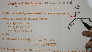
- Velocity Potential Functions: These functions represent the velocity field as gradients, simplifying the problem by reducing the number of variables from three (u, v, w) to one (phi).
- Irrotational Flow: Velocity potential functions are applicable only in irrotational flows, where the vorticity is negligible.
- Boundary Conditions: The derivation takes into account specific boundary conditions, such as no-slip conditions at the plate surfaces.
Deriving Simple Flow Solutions:
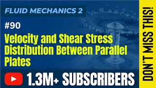
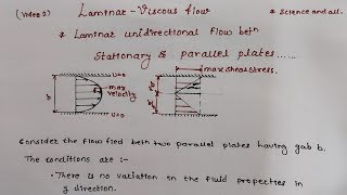
- Flow Between a Fixed and Moving Plate: By setting up the coordinate system and applying relevant approximations (e.g., neglecting gravity in horizontal flow), we derive the velocity distribution using continuity and momentum equations, ultimately arriving at a linear velocity profile.
- Flow Due to Pressure Gradient: For flow between two fixed plates influenced by a pressure gradient, we integrate the Navier-Stokes equations again, yielding a parabolic velocity profile representative of the pressure gradient influence.
Overall, this section integrates theoretical principles and practical derivations to strengthen understanding of fluid dynamics in engineering applications.
Youtube Videos


Audio Book
Dive deep into the subject with an immersive audiobook experience.
Introduction to Velocity Potentials
Chapter 1 of 4
🔒 Unlock Audio Chapter
Sign up and enroll to access the full audio experience
Chapter Content
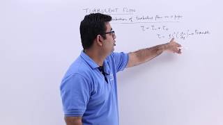
So basically let us start with Navier-Stokes equations which is long back about 200 years back. So the equations what we derive in last two classes we will go more detail about that. Before going that let me I just write down the basics equations is the Euler equations okay.
So if you look it when I talk about Euler equations you can understand it. It is for incompressibles and non-viscous or fixed or less flow. So this is the reasons we can apply it that means if you consider flow past a tall building okay a high rise buildings okay flow past tall building...
Detailed Explanation
The velocity potential is a mathematical function that helps simplify the analysis of fluid flow problems. By using velocity potentials, we can reduce the complexity of the equations we need to solve. For example, the Euler equations govern the motion of fluid under certain conditions, and when dealing with potential flows, we concentrate on the velocity being potentially derived from a single scalar function, rather than multiple components. This reduction allows for easier calculations, especially in fluid mechanics involving irrotational flows, where we can apply these potentials effectively.
Examples & Analogies
Imagine you are trying to navigate through a crowded room filled with people (the fluid). It could be complicated to measure the flow of each person (velocity components) individually. However, if you draw a map (the velocity potential function) that identifies the pathways and directions that will help most people move smoothly through the room (streamlines), you can better understand and predict how they will flow together through the crowd.
Conditions for Velocity Potential Functions
Chapter 2 of 4
🔒 Unlock Audio Chapter
Sign up and enroll to access the full audio experience
Chapter Content
Thus if I define it the velocity is a gradient of phi, phi is a velocity potential function at which condition thus this is what justified it was. If you look at the very basic components if I velocity potentials. v equal to grade phi is the gradient of a scalar components will be justified okay or the reverse is also true that when you have v is equal to 0 okay...
Detailed Explanation
To use velocity potentials effectively, specific conditions must be satisfied. Notably, it should be an irrotational flow, meaning there are no swirling movements within the fluid. Mathematically, we can represent the velocity (v) as the gradient of the potential function (phi). This means that to derive the velocity components in the fluid (u, v, w), we only need to calculate the derivatives of phi, rather than solve for each component separately. Therefore, if the flow is not irrotational, the concept of a velocity potential function does not apply.
Examples & Analogies
Consider a calm lake's surface on a peaceful day—there are no ripples or waves, representing an irrotational flow. If someone tosses a small stone (introducing a disturbance), you start to see ripples spreading out in circles. This scenario illustrates that as long as the lake is calm, we can utilize potential functions to describe what happens, but as soon as the water becomes turbulent, the situation requires a more complex analysis, illustrating why we need irrotational conditions.
Application in Streamline and Equipotential Lines
Chapter 3 of 4
🔒 Unlock Audio Chapter
Sign up and enroll to access the full audio experience
Chapter Content
Let me have a very simple way look at this relationship the orthogonality relationship it is not a big idea that you take a phi functions okay it is a line let me a two dimensional functions okay. So if you have a consider is phi is a constant and this line okay that is what along this velocity potential functions...
Detailed Explanation
Streamlines and equipotential lines provide visual tools to understand fluid flow. Streamlines represent the paths followed by fluid particles, while equipotential lines indicate points of constant potential function (phi). Importantly, where these two sets of lines intersect, they form right angles, which is a characteristic feature. This orthogonality means that we can effectively analyze flows; if we know the behavior along one set of lines, we can infer how it influences the other set, allowing for a deeper understanding of the fluid dynamics at play.
Examples & Analogies
Think about riding a bicycle on a countryside road versus through a valley surrounded by mountains. The road (streamlines) will direct how you can move while the valleys (equipotential lines) show the heights you might pass. Where the road intersects with the valleys, imagine being at a turn; you'll need to change directions, akin to the right angles formed in fluid flow. Therefore, understanding where these lines meet and how they influence each other can help you navigate smoothly through the landscape.
Summary of Key Concepts
Chapter 4 of 4
🔒 Unlock Audio Chapter
Sign up and enroll to access the full audio experience
Chapter Content
Now coming back to doing some simple approximations using Navier-Stokes equations to get simple solutions of between a fixed and moving plate viscous flow if you have we called cute flow okay. Conditions is that I have a fixed plate okay. So means the velocity is 0...
Detailed Explanation
In fluid mechanics, understanding how fluid behaves between fixed and moving surfaces is critical. By using the Navier-Stokes equations, we can derive the velocity distribution of fluid in this confined space. Certain assumptions, like neglecting gravity in horizontal flow, help simplify these complex equations into more manageable ordinary differential equations. By applying boundary conditions, such as knowing one plate is stationary and the other is moving, we can derive simple linear velocity profiles that represent how fluid flows under these constraints.
Examples & Analogies
Consider the gap between two slices of bread in a sandwich—one slice held still while you spread butter on the moving top slice. The butter (fluid) moves between the slices, and you can imagine the flow becoming easier and smoother as the top slice moves. When determining how fast the butter flows (melting and spreading) based on your spreading force, we use approximations similar to those applied in fluid mechanics when analyzing the flow between surfaces.
Key Concepts
-
Velocity Potential Functions: These functions represent the velocity field as gradients, simplifying the problem by reducing the number of variables from three (u, v, w) to one (phi).
-
Irrotational Flow: Velocity potential functions are applicable only in irrotational flows, where the vorticity is negligible.
-
Boundary Conditions: The derivation takes into account specific boundary conditions, such as no-slip conditions at the plate surfaces.
-
Deriving Simple Flow Solutions:
-
Flow Between a Fixed and Moving Plate: By setting up the coordinate system and applying relevant approximations (e.g., neglecting gravity in horizontal flow), we derive the velocity distribution using continuity and momentum equations, ultimately arriving at a linear velocity profile.
-
Flow Due to Pressure Gradient: For flow between two fixed plates influenced by a pressure gradient, we integrate the Navier-Stokes equations again, yielding a parabolic velocity profile representative of the pressure gradient influence.
-
Overall, this section integrates theoretical principles and practical derivations to strengthen understanding of fluid dynamics in engineering applications.
Examples & Applications
The velocity distribution between a fixed plate and a moving plate can be modeled linearly, whereas flow driven by a pressure gradient creates a parabolic velocity profile.
When fluid flows around objects, such as a tall building, differentiating between irrotational and rotational flow is essential for appropriate model application.
Memory Aids
Interactive tools to help you remember key concepts
Rhymes
In fluid motion, we must see, Navier's laws make it easy as can be!
Stories
Once a fluid raced between two plates, one fixed and one that skates. The velocity climbed from zero with glee, straight as an arrow, couldn't be dear.
Memory Tools
P.V.I. - Pressure, Velocity, Incompressibility - key factors in flow problems.
Acronyms
VISC
Viscosity
Incompressibility
Streamlines
Continuity - key aspects!
Flash Cards
Glossary
- NavierStokes Equations
A set of equations that describe the motion of fluid substances, accounting for viscosity and external forces.
- Velocity Potential Function
A scalar function whose gradient gives the velocity field, applicable in irrotational flow.
- Irrotational Flow
A flow where the vorticity is negligible, allowing for the use of velocity potential functions.
- Continuity Equation
An equation that states that mass is conserved in fluid flow; for incompressible flow, it ensures that the divergence of the velocity field is zero.
- Pressure Gradient
The rate of change of pressure in a fluid, which can drive flow.
Reference links
Supplementary resources to enhance your learning experience.