
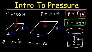
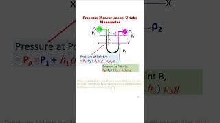
Pressure Field Calculations
Enroll to start learning
You’ve not yet enrolled in this course. Please enroll for free to listen to audio lessons, classroom podcasts and take practice test.
Interactive Audio Lesson
Listen to a student-teacher conversation explaining the topic in a relatable way.
Introduction to Navier-Stokes Equations
🔒 Unlock Audio Lesson
Sign up and enroll to listen to this audio lesson

Today, let's begin our discussion by revisiting the Navier-Stokes equations. These equations govern fluid motion and are fundamental to fluid mechanics. Can anyone tell me what controls complex fluid flow?

Is it the forces acting on the fluid like pressure gradients?
Exactly! The balance between pressure gradients, viscous forces, and inertia dictates flow behavior. Remember: 'VPI' - Viscous forces, Pressure gradients, Inertial forces are key in Navier-Stokes equations.

What’s the significance of deriving Bernoulli's equations from these?
Great question! Bernoulli’s equation simplifies the analysis of fluid flow, especially for incompressible and non-viscous flows, by reducing complexity.

Can we use it for all kinds of fluid flow?
Not necessarily, Bernoulli's can only be applied in idealized conditions. We will cover more examples during this session.

Wait! What’s this 'irrotational flow'?
Irrotational flow means there’s no vorticity in the fluid. It’s essential when applying velocity potential functions. Let's explore these concepts deeper now.
Velocity Potentials and Their Applications
🔒 Unlock Audio Lesson
Sign up and enroll to listen to this audio lesson

Now, let's talk about velocity potentials. This amazing single scalar function, phi, helps us express three velocity components succinctly.
How do we derive the velocity components from phi?
Excellent! You derive components by taking partial derivatives of phi. For example, u = ∂phi/∂x, v = ∂phi/∂y, and w = ∂phi/∂z.
And this is applicable when the flow is irrotational, right?
Yes! In irrotational flow, no rotation occurs around any point; hence, we can express the flow simply using phi.
So that’s where we use the Laplacian of phi too?
Correct! The Laplacian helps us connect the scalar potential field to hydrostatic equilibrium, facilitating easier calculations.
Viscous Flow Between Plates
🔒 Unlock Audio Lesson
Sign up and enroll to listen to this audio lesson
Let’s delve into viscous flow, particularly between fixed and moving plates. What do we need to consider in these scenarios?
We need the Navier-Stokes equations for the calculations, right?
Exactly! In this case, we simplify by neglecting gravity and considering steady flow conditions. This reduces the complexity of the system.
So, we end up with simpler ordinary differential equations?
Precisely! We can integrate these equations under specified boundary conditions to determine velocity distributions.
What about the pressure gradient?
Great point! The pressure gradient affecting the flow is crucial in determining how velocity varies particularly in scenarios like these.
Pressure Field Calculations and Implications
🔒 Unlock Audio Lesson
Sign up and enroll to listen to this audio lesson
Now, let's link pressure fields with our earlier discussions. How would you approach determining the pressure field for our fluid scenario?
I suppose we would apply the Navier-Stokes equations and continuity conditions?
That's a solid plan! Remember to check if the velocity fields satisfy continuity first. It's a key step.
Could you summarize how we connect all this?
Certainly! By using velocity potentials and analyzing the Navier-Stokes equations, we establish relations among pressures, velocities, and flow characteristics. Recap with the acronym ‘VPI’ again!
Introduction & Overview
Read summaries of the section's main ideas at different levels of detail.
Quick Overview
Standard
In this section, we explore derivations from Navier-Stokes equations to obtain velocity potentials and their relationship to pressure fields in fluid flow. We discuss the implications of irrotational flow and pressure gradients in determining velocity distributions between fixed and moving plates.
Detailed
Detailed Summary
This section delves into the calculations of pressure fields using Navier-Stokes equations within the context of fluid mechanics. It begins with a review of basic principles, emphasizing the derivation of Bernoulli's equations from the Navier-Stokes framework. The concept of velocity potential functions is introduced, highlighting their role in simplifying flow problems by reducing three velocity components into a single scalar function, phi. The conditions under which velocity potential functions are applicable, particularly in irrotational flow contexts, are explored thoroughly.
Subsequently, the text outlines methods to analyze incompressible viscous flow scenarios, particularly focusing on flow characteristics between fixed and moving plates. Approximations made in these calculations include the neglect of gravitational forces and pressure gradients in specific cases, leading to simplified ordinary differential equations that describe the flow. The significance of continuity equations and their satisfaction by the imposed velocity fields is emphasized to ascertain valid pressure field calculations. Overall, the content elucidates foundational fluid mechanics concepts that underpin various applications in civil engineering.
Youtube Videos
![Introduction to Velocity Fields [Fluid Mechanics #1]](https://img.youtube.com/vi/CkNo5xGMZS4/mqdefault.jpg)
![[CFD] The PISO Algorithm](https://img.youtube.com/vi/ahdW5TKacok/mqdefault.jpg)

Audio Book
Dive deep into the subject with an immersive audiobook experience.
Overview of Pressure Field Calculations
Chapter 1 of 5
🔒 Unlock Audio Chapter
Sign up and enroll to access the full audio experience
Chapter Content
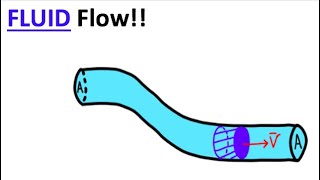
In this section, we are looking to compute the pressure field using the continuity and Navier-Stokes equations. We will analyze a steady, two-dimensional incompressible flow where the given velocity components fulfill the criteria for fluid flow.
Detailed Explanation
This chunk introduces the main objective of the section: to compute the pressure field in a fluid under certain conditions. To achieve this, we will use the continuity equations and Navier-Stokes equations that govern fluid dynamics. The context is a steady, two-dimensional incompressible flow, which simplifies the analysis by reducing the number of variables we need to consider.
Examples & Analogies
Think of this like trying to find out how much pressure is behind a flowing river. To do this, we need to understand how the water is moving (velocity) and ensure that nothing's obstructing it (continuity). Just as a steady current in the river pushes downstream smoothly, our flow must also be stable and consistent.
Continuity Equations and Velocity Fields
Chapter 2 of 5
🔒 Unlock Audio Chapter
Sign up and enroll to access the full audio experience
Chapter Content
To check if the velocity field fits the requirements for fluid flow, we will ensure that the continuity equation is satisfied, which states that the sum of the rates of flow into a junction must equal the rates of flow out.
Detailed Explanation
The continuity equation plays a crucial role in fluid mechanics, ensuring conservation of mass. For a two-dimensional incompressible flow, this means that the change in velocity in one direction must be balanced by corresponding changes in other directions. In our case, we check the given velocity components against these requirements. If they meet the continuity condition, we can proceed to derive the pressure field.
Examples & Analogies
Imagine a water hose: if the hose is narrow at one end, the water must move faster through that section to keep the flow steady. If we consider different widths along the hose, the consistency of the water flow must remain balanced. This analogy helps illustrate the continuity definition applied here.
Navier-Stokes Equations in Two-Dimensional Flow
Chapter 3 of 5
🔒 Unlock Audio Chapter
Sign up and enroll to access the full audio experience
Chapter Content
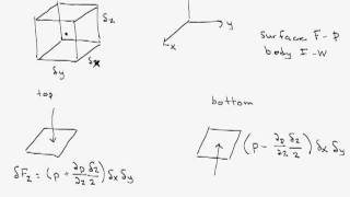
With the continuity equation satisfied, we will apply the two-dimensional Navier-Stokes equations. This mathematical tool helps us relate the motion of fluid elements to changes in pressure.
Detailed Explanation
The Navier-Stokes equations describe how the velocity field in a fluid evolves over time, incorporating various forces such as pressure, viscous effects, and sometimes external forces like gravity. In the context of our two-dimensional flow, we simplify these equations by excluding components that are zero (like gravity in horizontal flow). By doing so, we can isolate the effects of pressure gradients on fluid motion and predict how pressure varies across the flow.
Examples & Analogies
Think of a flat piece of paper that's being pushed through a fluid (like syrup). The way the paper moves through the syrup relates closely to how pressure affects the fluid around it. If the pressure behind the paper is higher than out front, the paper will move forward; thus, the Navier-Stokes equations help us quantify these relationships.
Pressure Field Calculation Steps
Chapter 4 of 5
🔒 Unlock Audio Chapter
Sign up and enroll to access the full audio experience
Chapter Content
To compute the pressure field, we simplify our equations, look at changes in velocities, and integrate them to find a smooth pressure function that characterizes the flow.
Detailed Explanation
Calculating the pressure field involves integrating our simplified forms of the Navier-Stokes equations. We ensure that the resulting pressure function remains continuous without any sudden changes. The integration gives us constants that we can solve using boundary conditions defined by our flow situation (like fixed points at the edges of our system). The result is a pressure field that can vary with the spatial coordinates in our flow domain.
Examples & Analogies
Picture blowing up a balloon. As you blow air into it, the pressure inside the balloon increases smoothly. If you could see the air's internal pressure changes as you blow, it would help you understand how pressure builds up within the confined space of the balloon, similar to how we analyze fluid pressures here.
Determining Flow Characteristics
Chapter 5 of 5
🔒 Unlock Audio Chapter
Sign up and enroll to access the full audio experience
Chapter Content
Once we have the pressure field, we can also determine additional characteristics of the flow, such as wall shear stress, stream functions, vorticity, and average velocity.
Detailed Explanation
The pressure field derived from our calculations allows us to evaluate various physical characteristics of the flow, providing insights into how the fluid behaves. For instance, wall shear stress gives us information about the force exerted by the fluid on the walls of the container or pipeline it flows through. Stream functions and vorticity describe how fluid traces move and rotate, enriching our understanding of the flow dynamics.
Examples & Analogies
Imagine flowing oil through pipes in a factory. Knowing the pressure allows engineers to predict how much oil can flow, how it will interact with the pipe walls (shear stress), and whether any turbulent eddies will form. Understanding these dynamics is crucial for designing efficient and safe transport systems.
Key Concepts
-
Navier-Stokes Equations: Fundamental equations governing fluid motion.
-
Irrotational Flow: Flow condition where vorticity is zero.
-
Velocity Potentials: Scalar functions defining fluid velocity.
-
Continuity Equation: Equation ensuring mass conservation in fluid systems.
-
Pressure Gradients: Influence fluid motion; derived from fluid forces.
Examples & Applications
Calculating pressure in a pipe using fluid velocity and height difference.
Analyzing pressure fields around a moving object using Navier-Stokes equations.
Memory Aids
Interactive tools to help you remember key concepts
Rhymes
In Navier-Stokes we trust, flows smooth and just; when vorticity is zero, potential functions are our hero.
Stories
Imagine a river with no ripples, flowing smoothly. It's like our ideal fluid where irrotational flow holds, and we derive the potential from phi.
Memory Tools
Remember 'VIP' for Navier-Stokes: Viscosity, Inertia, Pressure for fluid flow analysis.
Acronyms
ZPV
Zero Vorticity implies Potential functions lead; without gravity
we simplify the need.
Flash Cards
Glossary
- NavierStokes Equations
A set of equations that describe the motion of fluid substances, considering elements like viscosity and pressure.
- Irrotational Flow
A flow condition where the vorticity of the fluid is zero; the flow can be described using velocity potentials.
- Velocity Potential
A scalar function whose gradient gives the velocity field in irrotational flow.
- Continuity Equation
A mathematical statement that signifies mass conservation in fluid flow.
- Pressure Gradient
A change in pressure per unit distance, influencing fluid motion.
Reference links
Supplementary resources to enhance your learning experience.