
Boundary Layer Approach Equations
Enroll to start learning
You’ve not yet enrolled in this course. Please enroll for free to listen to audio lessons, classroom podcasts and take practice test.
Interactive Audio Lesson
Listen to a student-teacher conversation explaining the topic in a relatable way.
Introduction to Boundary Layer Approach
🔒 Unlock Audio Lesson
Sign up and enroll to listen to this audio lesson

Good morning, everyone! Today we are going to discuss the boundary layer approach in fluid mechanics. Has anyone heard about boundary layers before?

Yes, I think it has something to do with how fluids behave near surfaces.
Exactly! The boundary layer is a thin region near a surface where the effects of viscosity are significant. In this section, we will link this concept to the Navier-Stokes equations. Can anyone tell me what the Navier-Stokes equations primarily describe?

They describe the motion of viscous fluids, right?
Correct! They're essential for analyzing fluid dynamics. Remember, we can derive simpler equations if we utilize velocity potentials in irrotational flows. Think of this like simplifying complex problems into manageable forms.

How do we determine if the flow is irrotational?
Good question! A flow is considered irrotational if the curl of the velocity field is zero. This is a key condition we need to assess. Let's summarize: boundary layers affect fluid behavior, and Navier-Stokes equations help analyze these behaviors in viscous flows.
Velocity Potentials and their Application
🔒 Unlock Audio Lesson
Sign up and enroll to listen to this audio lesson

Moving on, let's talk about velocity potentials! Can anyone explain what a velocity potential function is?

It's a scalar function used to describe the flow field, right?
Exactly! We denote it as φ. For a flow where the velocity is irrotational, the velocity vector is equal to the gradient of this potential function: v = ∇φ. Does this make sense?
So, instead of dealing with multiple velocity components, we can just use one scalar function?
Yes, and this greatly simplifies our analysis. The potential function varies with space and time, helping predict how the fluid behaves in complex scenarios.
What kind of conditions must be met for using this function?
Good insight! The conditions include an irrotational flow and the absence of significant turbulence or vorticity in the analyzed region. Let's wrap this session up: velocity potentials help us simplify and solve fluid dynamics problems effectively.
Applications of Navier-Stokes equations
🔒 Unlock Audio Lesson
Sign up and enroll to listen to this audio lesson
Now, let's apply our knowledge to some real-world scenarios. Can anyone think of where we might use the Navier-Stokes equations?
I think they are used for analyzing flow past buildings.
Absolutely! For instance, when studying wind flow around tall buildings, we examine how the flow separates and generates vortices. In these cases, the Euler equations may be applicable outside the boundary layer.
What do you mean by pressure gradients affecting flow?
The pressure gradient drives the flow. In a simplified case, such as fluid between two plates with a pressure drop, Navier-Stokes helps us model the velocity distribution across the gap.
So, we can use these equations to predict how fast the fluid will flow between those plates?
Exactly! Recap: the Navier-Stokes equations help describe fluid motion under various conditions, which is essential in engineering applications.
Transition from Irrotational to Rotational Flow
🔒 Unlock Audio Lesson
Sign up and enroll to listen to this audio lesson
Let's explore how flows transition from irrotational to rotational. What factors might contribute to this change?
I think if there are solid boundaries or significant turbulence, the flow can become rotational.
Exactly! Viscosity plays a crucial role here. When the flow encounters objects, such as when air moves past a building, it generates vorticity, making the flow rotational.
Is it true that Bernoulli’s equation can't be used in such situations?
Correct! When viscosity dominates, the simplifications of Bernoulli's equation become invalid. Thus, understanding these transitions is vital. Summary: flow can shift from irrotational to rotational due to boundaries, vorticity, or pressure gradients.
Introduction & Overview
Read summaries of the section's main ideas at different levels of detail.
Quick Overview
Standard
In this section, we explore the boundary layer approach in fluid mechanics, focusing on the application of the Navier-Stokes equations, Euler equations, and the concept of velocity potential functions. The relationship between irrotational flow and boundary layer formation, along with practical examples, illustrates how these theories are applied to real-world fluid flow problems.
Detailed
Boundary Layer Approach Equations
In this section, we delve into the boundary layer approach to understanding fluid dynamics by discussing key equations such as the Navier-Stokes and Euler equations. The Navier-Stokes equations describe motion in viscous fluids and can be simplified under certain assumptions. In the scope of this section, we particularly focus on:
- Velocity Potentials: This concept helps simplify the flow analysis by allowing us to use scalar functions to represent the flow field instead of multiple velocity components. The velocity potential function (denoted as φ) is linked with irrotational flow, where the fluid motion can be expressed through the gradient of φ. This simplification is effective only in regions where the flow is irrotational.
- Irrotational vs. Rotational Flows: We discuss the conditions under which fluids transition from irrotational to rotational flow, particularly emphasizing the influence of forces such as viscosity, solid boundaries, and pressure gradients.
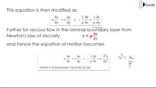
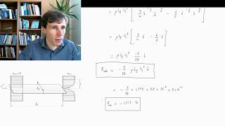
- Practical Applications: Through examples, we demonstrate how to apply the Navier-Stokes equations for specific cases, including flow between fixed and moving plates. The boundary layer approximation allows us to identify velocity distributions and shear stress distributions within these flows, enhancing our understanding of real-world applications in engineering structures such as high-rise buildings and flow past surfaces.
By the end of this section, readers should recognize the significance of the boundary layer equations and how simplifying assumptions affect fluid flow models in engineering contexts.
Youtube Videos


Audio Book
Dive deep into the subject with an immersive audiobook experience.
Introduction to Boundary Layer Approximations
Chapter 1 of 4
🔒 Unlock Audio Chapter
Sign up and enroll to access the full audio experience
Chapter Content
Good morning all of you. Today we are going to discuss about approximation solutions of Navier-Stokes equations. That is what we earlier started, to how to approximate the Navier-Stokes equation for simple problems flow through two plates with movable plate with pressure gradient.
Detailed Explanation
In the beginning of this lecture, the instructor sets the stage for discussing boundary layer approximations in fluid mechanics. They mention that these approximations will focus on solutions to the Navier-Stokes equations, which describe the motion of fluid substances. The goal is to simplify these complex equations to analyze flow in practical scenarios, like the flow between two plates. By making reasonable assumptions about how fluids behave, we can arrive at simpler models that still provide accurate solutions for many types of fluid flow problems.
Examples & Analogies
Imagine a stream where the middle flows freely while the edges are slowed down by the riverbank. The middle part can be approximated simply, while the edges require a careful examination to understand their slower speed. This analogy helps visualize what boundary layer approximations do — simplify the model to focus on the main parts of the flow.
Conditions for Steady, Incompressible Flow
Chapter 2 of 4
🔒 Unlock Audio Chapter
Sign up and enroll to access the full audio experience
Chapter Content
The problem is that there is a steady again I am emphasizing two-dimensional incompressible velocity field is given to us. We have to compute a functions pressure is a function of x and y.
Detailed Explanation
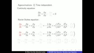
The instructor clarifies that a steady, two-dimensional, incompressible flow must be analyzed. This means the flow properties do not change over time, and the fluid density remains constant. The goal is to compute pressure variations based on two spatial dimensions, x and y. This sets the foundation for deriving pressure from the given velocity field. The continuity equation will be used to ensure that the velocity field adheres to the principles of fluid flow, which requires that fluids exiting a region are equal to fluids entering it.
Examples & Analogies
Think of a crowded marketplace: a constant number of people (representing fluid mass) are entering and exiting. If more people enter than exit, you will have a buildup. The continuity equation ensures that the flow into a section equals the flow out, similar to balancing people in and out of a market.
Continuity Equation Satisfaction
Chapter 3 of 4
🔒 Unlock Audio Chapter
Sign up and enroll to access the full audio experience
Chapter Content
Now we are looking it whether what is a pressure field we have to compute it which will be a function of as a 2-dimensional flow, steady 2-dimensional incompressible flow.
Detailed Explanation
The continuity equation for two-dimensional incompressible flow must be satisfied. The instructor checks whether the derived velocity components meet this requirement. If they do not, the pressure field cannot be computed as it indicates a non-physical situation. The continuity equation specifically requires that the sum of changes in the flow direction be zero, ensuring no accumulation of mass in any section of the fluid.
Examples & Analogies
Imagine a water slide where kids are constantly entering and exiting the water. If too many kids are trying to enter the slide at the same time, congestion occurs, and some would have to wait. The continuity equation ensures that the number of kids in the slide remains constant, just like the fluid flow needs to maintain a balance.
Deriving Pressure from Navier-Stokes Equations
Chapter 4 of 4
🔒 Unlock Audio Chapter
Sign up and enroll to access the full audio experience
Chapter Content
If the velocity field does not satisfy the continuity equation, we should not find out the pressure field for that. So as the flow fluid, we have a continuity equation, so we have an eviscerative equation.
Detailed Explanation
After confirming that the velocity satisfies the continuity equation, the next step is to apply the Navier-Stokes equations to derive the pressure field. The instructor highlights the importance of clearly writing the equations, taking into account that the pressure must comply with fluid dynamics principles. The equations will reveal how pressure changes with respect to the flow, considering all the influences like gravity and fluid viscosity.
Examples & Analogies
Think of pressure in a water balloon: if the amount of water (mass flow) is constant, any increase in the squeeze from the outside (pressure) must change the flow inside. The instructor demonstrates how similar relationships are at play when calculating pressure changes in fluid dynamics.
Key Concepts
-
Boundary Layer: A region near a surface significantly affected by viscous forces.
-
Navier-Stokes Equations: Fundamental equations governing fluid motion in viscous flows.
-
Velocity Potential: A scalar function representing fluid motion in irrotational flows.
-
Irrotational Flow: A state of flow with no vorticity, allowing simplifications in fluid mechanics.
Examples & Applications
High-rise buildings experiencing wind shear, modeled using the Navier-Stokes equations to understand flow separation.
Velocity distributions in fluid flow between two parallel plates analyzed through boundary layer theory.
Memory Aids
Interactive tools to help you remember key concepts
Rhymes
In layers thin and close to skin, viscosity plays right where we begin.
Stories
Imagine a river meeting a rock; the water slows down at the edge, creating a layer where the motion is different from the fast-moving center, just like a boundary layer.
Memory Tools
Use the acronym 'IRV' to remember: 'I' for Irrotational flow, 'R' for Rotational flow, 'V' for Velocity potentials.
Acronyms
BL for Boundary Layer
remember
it's where viscosity is a significant player!
Flash Cards
Glossary
- Boundary Layer
A thin region adjacent to a surface where the effects of viscosity significantly impact the fluid flow.
- NavierStokes Equations
A set of nonlinear partial differential equations that describe the motion of viscous fluid substances.
- Velocity Potential Function
A scalar function whose gradient yields the velocity field in irrotational flow.
- Irrotational Flow
A fluid flow condition characterized by the absence of vorticity, where the curl of the velocity field is zero.
- Rotational Flow
Fluid flow that involves vorticity and turbulence, causing non-uniformity in velocity distribution.
Reference links
Supplementary resources to enhance your learning experience.