
Gram-Schmidt Process
Enroll to start learning
You’ve not yet enrolled in this course. Please enroll for free to listen to audio lessons, classroom podcasts and take practice test.
Interactive Audio Lesson
Listen to a student-teacher conversation explaining the topic in a relatable way.
Understanding Orthogonal Vectors
🔒 Unlock Audio Lesson
Sign up and enroll to listen to this audio lesson

Today, we're going to explore the concept of orthogonal vectors. Can anyone tell me what we mean when we say two vectors are orthogonal?

I think it means they are at right angles to each other.
Exactly! Two vectors are orthogonal if their dot product is zero, which geometrically represents them being at right angles. If vector u and vector v satisfy u·v = 0, they are orthogonal.

So, they don't influence each other in terms of direction?
That's correct! And they form an orthonormal set when all vectors in the group have a magnitude of one. Remember, orthogonality means independence which simplifies many calculations.

Interesting! Why is this important in engineering?
In engineering, especially civil engineering, we use these concepts to simplify complex mathematical problems. For instance, orthogonal vectors help in numerical simulations where clear and independent axes of application are needed.
To sum up, orthogonal vectors are key to ensuring that computations and analyses remain straightforward and efficient.
Introduction to the Gram-Schmidt Process
🔒 Unlock Audio Lesson
Sign up and enroll to listen to this audio lesson

Now that we understand orthogonal vectors, let’s dive into the Gram-Schmidt Process. Who can explain why we would want to use this process with our set of vectors?
So we can turn any linearly independent set into an orthonormal set?
Exactly! The Gram-Schmidt Process allows us to take a set of linearly independent vectors and convert them into orthonormal vectors, a crucial step in many mathematical applications.

What are the steps involved in this process?
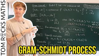
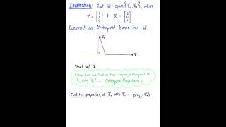
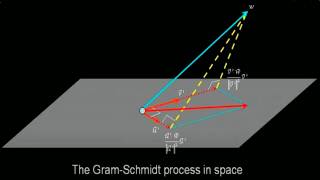
Great question! The process consists of the following key steps: First, start with your first vector and normalize it; this is your first orthonormal vector. Then, for each subsequent vector, subtract the projections onto the already created orthonormal vectors and normalize the result. Let’s visualize this process on the board.
That sounds quite practical! Can we use it in real applications?
Absolutely. For example, in civil engineering, when we're modeling structures, we need an orthonormal set to simplify complex calculations, ensuring numerical stability and good accuracy in solutions.
In summary, the Gram-Schmidt Process not only provides the necessary orthogonalization of vectors but also enhances the computational efficiency across various applications.
Introduction & Overview
Read summaries of the section's main ideas at different levels of detail.
Quick Overview
Standard
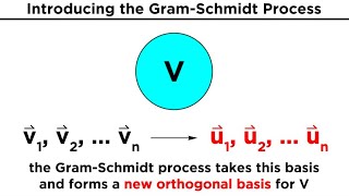
The Gram-Schmidt Process involves taking a set of linearly independent vectors and transforming them into an orthonormal basis for a vector space. This process is essential in various fields, including civil engineering, where orthogonal vectors simplify computations in linear algebra applications.
Detailed
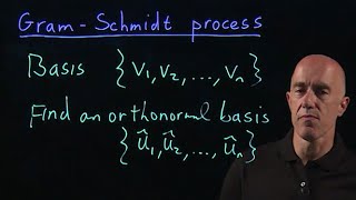
Gram-Schmidt Process
The Gram-Schmidt Process is an algorithm that transforms a set of linearly independent vectors into an orthonormal set, which means the vectors are not only independent but also orthogonal and unit vectors (having a norm of one). This technique is particularly significant in linear algebra as it simplifies solving systems of equations and helps in numerical computations where orthonormal bases are required.
Key Points Cover:
- Orthogonal Vectors: Vectors that meet the condition of having a dot product equal to zero, i.e., if vectors u and v are orthogonal, then u·v = 0.
- Orthonormal Set: This is a set where the vectors are orthogonal and also unit vectors (each having a magnitude of 1).
- Application: The Gram-Schmidt Process is often utilized in numerical analysis, particularly in methods related to finite element analysis and other computational techniques in civil engineering, ensuring stability and accuracy of the solutions derived from linear algebraic methods.
Youtube Videos
Audio Book
Dive deep into the subject with an immersive audiobook experience.
Orthogonal Vectors
Chapter 1 of 4
🔒 Unlock Audio Chapter
Sign up and enroll to access the full audio experience
Chapter Content
Two vectors u and v are orthogonal if:
$$u·v = 0$$
Detailed Explanation
Orthogonal vectors are those that meet at a right angle, which means that when you find the dot product of the two vectors, the result is zero. Mathematically, this is expressed as u·v = 0. If you visualize vectors as arrows in space, two orthogonal vectors would look like the arms of a cross or the axes of a graph, where they intersect perpendicularly.
Examples & Analogies
Imagine a basketball court: the two lines at the center form a right angle. One line represents the baseline, and the other the sideline. The players moving along these lines are operating in orthogonal directions.
Orthonormal Set
Chapter 2 of 4
🔒 Unlock Audio Chapter
Sign up and enroll to access the full audio experience
Chapter Content
A set of vectors that are both orthogonal and unit vectors.
Detailed Explanation
An orthonormal set is a collection of vectors that not only are orthogonal to each other but also have a length (or magnitude) of one. This means you can easily calculate angles and projections since each vector's influence is standardized to a unit length. This is particularly useful in computing and mathematical modeling, simplifying operations involving these vectors.
Examples & Analogies
Think of a team of assistants at a conference, where each assistant is responsible for a specific area (orthogonality). If they each stand exactly one meter apart, ready to handle their tasks, they form an orthonormal set, making coordination easier.
Gram-Schmidt Process
Chapter 3 of 4
🔒 Unlock Audio Chapter
Sign up and enroll to access the full audio experience
Chapter Content
A method to convert a set of linearly independent vectors into an orthonormal set.
Detailed Explanation
The Gram-Schmidt Process is a systematic method for taking a group of linearly independent vectors and transforming them into a new orthonormal set. This process involves orthogonalizing the vectors step by step and normalizing them to ensure each one has a unit length. The result is that you can perform calculations more easily and accurately in vector spaces due to the orthonormal properties achieved.
Examples & Analogies
Imagine sculpting a statue. You start with a block of raw marble (linearly independent vectors) and, through careful chiseling (the Gram-Schmidt Process), you produce a series of refined pieces of art (orthonormal set). Each piece is not only distinct but easy to place together into a beautiful integrated whole.
Applications of Gram-Schmidt Process
Chapter 4 of 4
🔒 Unlock Audio Chapter
Sign up and enroll to access the full audio experience
Chapter Content
Applications
- Numerical solutions of partial differential equations.
- Finite element methods in structural analysis.
Detailed Explanation
The Gram-Schmidt process has practical applications in many areas, particularly in numerical methods for solving complex equations. For instance, in structural analysis, elements such as beams and trusses can be modeled using matrices where the Gram-Schmidt process helps in simplifying the calculations, leading to more efficient and accurate modeling. In numerical solutions of partial differential equations, having an orthonormal set significantly aids in convergence and stability of the solution.
Examples & Analogies
Think of constructing a bridge: engineers must ensure each segment is not only strong but harmonizes with others. Using the Gram-Schmidt process is akin to ensuring each part of the construction fits perfectly without misalignments, allowing for a safer, more robust design.
Key Concepts
-
Orthogonal Vectors: Vectors that meet the condition of having a dot product equal to zero.
-
Orthonormal Set: A set where the vectors are orthogonal and also unit vectors.
-
Gram-Schmidt Process: An algorithm that converts a set of linearly independent vectors into an orthonormal set.
Examples & Applications
Consider vectors A = (1, 2) and B = (2, -1). To check if they are orthogonal, we compute A·B = 12 + 2(-1) = 0, hence they are orthogonal.
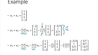
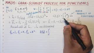
Given two linearly independent vectors in R^3, e.g., v1 = (1, 0, 0) and v2 = (1, 1, 0). Applying the Gram-Schmidt Process, we can create an orthonormal set by normalizing v1 and projecting v2 onto v1.
Memory Aids
Interactive tools to help you remember key concepts
Rhymes
Orthogonality is key, it's where vectors agree, zero dot product, as simple as can be!
Stories
Imagine vectors as friends at a party. Two friends don't disturb each other—that's orthogonal. They are all well-behaved, just like orthonormal vectors with unity in their length!
Memory Tools
O1N stands for 'Orthogonal and 1 Norm,' a way to remember Orthonormal vectors.
Acronyms
GSP - Gram-Schmidt Process
Get them Orthonormal
Separate by projecting!
Flash Cards
Glossary
- Orthogonal Vectors
Vectors that are perpendicular to each other, resulting in a dot product of zero.
- Orthonormal Set
A set of vectors that are both orthogonal and of unit length.
- GramSchmidt Process
A method for converting a linearly independent set of vectors into an orthonormal set.
- Projection
The component of one vector along the direction of another vector.
Reference links
Supplementary resources to enhance your learning experience.