
Matrix Representation
Enroll to start learning
You’ve not yet enrolled in this course. Please enroll for free to listen to audio lessons, classroom podcasts and take practice test.
Interactive Audio Lesson
Listen to a student-teacher conversation explaining the topic in a relatable way.
Introduction to Linear Transformations
🔒 Unlock Audio Lesson
Sign up and enroll to listen to this audio lesson

Today, we're discussing linear transformations, which map vectors from one space to another while preserving structure. Can anyone tell me what defines a linear transformation?

Is it something that keeps both addition and scalar multiplication?
Exactly! We have: T(u + v) = T(u) + T(v) and T(cu) = cT(u). These properties ensure the transformation is linear. Now, if we have a transformation T: V → W, how would we represent it using matrices?

Are we saying T(x) = Ax, where A is the matrix?
Yes, very good! The matrix A enables us to perform operations on the input vector x conveniently. Let's remember that A captures all transformation behavior. Now, what could be the implications of linear transformations in engineering?

They help simplify complex structures and models, right?
Right! They play a crucial role in simulations and structural analysis.
Kernel and Range
🔒 Unlock Audio Lesson
Sign up and enroll to listen to this audio lesson

Now let's discuss two crucial concepts: kernel and range. Can anyone explain what the kernel is?

Isn't it the set of vectors in V that get mapped to zero in W?
Exactly! This set tells us about solutions to the homogeneous equations. What about the range?
The range is the collection of all images produced by T from inputs in V.
Correct! The range helps us understand the output space of a transformation. Now, how do these concepts relate to the Rank-Nullity Theorem?
It states the dimension of the kernel plus the dimension of the range equals the dimension of the domain!
You’ve got it! This theorem helps us analyze linear transformations effectively.
Applications of Matrix Representation
🔒 Unlock Audio Lesson
Sign up and enroll to listen to this audio lesson
Let's now explore how matrix representation impacts civil engineering. Why do you think we need matrix representations in engineering?
They help in analyzing structures through transformations, right?
Absolutely! They are crucial for simulations, stress analysis, and coordinate transformations. Can anyone think of specific engineering problems that use these concepts?
I think the analysis of forces in trusses can utilize these transformations.
Great example! It's fundamental in structural integrity assessments. Remember, understanding these transformations helps in optimizing designs.
Introduction & Overview
Read summaries of the section's main ideas at different levels of detail.
Quick Overview
Standard
Matrix representation is crucial for understanding linear transformations between vector spaces. It involves expressing linear transformations in a matrix form, analyzing the kernel and range, and applying the Rank-Nullity Theorem to connect these concepts, which are essential in various applications, including engineering.
Detailed
Matrix Representation
In this section, we delve into the concept of matrix representation of linear transformations. A linear transformation from vector space V to vector space W is defined as a map T: V → W that conserves vector addition and scalar multiplication properties:
- T(u+v) = T(u) + T(v)
- T(cu) = cT(u)
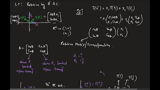
Every linear transformation can be represented as a matrix acting upon a vector. This is expressed in the format T(x) = Ax, where A is the matrix associated with the transformation and x is the vector. The process of converting a linear transformation into its matrix form is pivotal in applications such as computational solutions in civil engineering and other mathematical fields.
Two critical concepts in this context are:
- Kernel (Null Space): This is the set of all vectors from V that are mapped to the zero vector in W under the transformation T. It reflects the solution set of homogeneous equations associated with the transformation.
- Range (Image): This is the collection of all possible outputs (or images) in W that can be produced via the transformation from any input vector in V. Understanding both the kernel and range of a matrix helps in analyzing its properties and the transformation it represents.
An important theorem related to this is the Rank-Nullity Theorem, which states that the dimensions of the kernel and range together must equal the dimension of the domain:
$$ \text{dim(Ker(T))} + \text{dim(Im(T))} = \text{dim(Domain)} $$
This relationship provides essential insight into the structure of linear mappings, allowing engineers and mathematicians alike to predict behavior in complex systems.
Youtube Videos
Audio Book
Dive deep into the subject with an immersive audiobook experience.
Definition of Linear Transformation
Chapter 1 of 5
🔒 Unlock Audio Chapter
Sign up and enroll to access the full audio experience
Chapter Content
A linear transformation T :V →W between two vector spaces satisfies:
T(u+v)=T(u)+T(v), T(cu)=cT(u)
Detailed Explanation
A linear transformation is a special type of mapping between two vector spaces. It has two main properties:
1. Additivity: This means that if you take two vectors, u and v, and add them together, the transformation of that sum is the same as transforming each vector separately and then adding the results. So, T(u + v) is equal to T(u) + T(v).
2. Homogeneity: This property states that if you multiply a vector (u) by a scalar (c), the transformation of that product is equal to multiplying the transformation of the vector by that scalar. Thus, T(cu) equals cT(u). These properties ensure that linear transformations have a structured behavior that is predictable and consistent across the vector spaces involved.
Examples & Analogies
Imagine you are a chef in a kitchen. If you add ingredients (like vegetables and spices) to a pot (like adding vectors), the final dish (the output) depends just on the ingredients you added, not on the order you added them (this represents additivity). Similarly, if you double the amount of chili peppers you add, the spiciness of the dish will also double (representing homogeneity). This structured behavior of combining and scaling ingredients mirrors how linear transformations work with vectors.
Matrix Representation of Linear Transformations
Chapter 2 of 5
🔒 Unlock Audio Chapter
Sign up and enroll to access the full audio experience
Chapter Content
Every linear transformation can be represented as a matrix acting on a vector:
T(x)=Ax
Detailed Explanation
In linear algebra, we can represent linear transformations using matrices. Suppose we have a linear transformation T that maps vectors from one vector space (V) to another (W). Instead of dealing with the transformation directly, we can associate it with a matrix A. If you have a vector x in space V, you can express the transformation of x using the matrix A as T(x) = Ax. This notation implies that the effect of the transformation T on the vector x can be calculated by multiplying the matrix A by the vector x. This approach allows us to leverage matrix operations to study and calculate various properties of the linear transformation more easily.
Examples & Analogies
Think of a linear transformation like a factory process where a machine represents the matrix A. The raw materials entering the machine are analogous to the vector x. As the materials go through the machine (matrix), they get processed, resulting in a finished product (the output of the transformation, T(x)). Just as you can adjust machine settings to change the output while keeping the process consistent, using matrices allows us to systematically handle transformations and easily compute their outcomes.
Kernel and Range
Chapter 3 of 5
🔒 Unlock Audio Chapter
Sign up and enroll to access the full audio experience
Chapter Content
Kernel (Null Space): Set of all vectors mapped to 0.
Range (Image): Set of all vectors that are images under T.
Detailed Explanation
In the context of linear transformations, two important concepts arise: the kernel and the range.
1. Kernel (Null Space): This set includes all vectors in the domain that are transformed into the zero vector in the codomain. If T(x) = 0, then x is part of the kernel. This helps us find vectors that lose their magnitude or are perfectly canceled out by the transformation.
2. Range (Image): This refers to the set of all possible output vectors that can be produced by the transformation T. Essentially, it encompasses all the vectors that can be expressed as T(x) for some x in the domain. Understanding the range helps us determine how expansive or limited the transformation is in covering the codomain.
Examples & Analogies
Imagine you are conducting an experiment in a lab where you mix chemicals (the vectors in the domain). The 'Kernel' would represent all the combinations of chemicals that cancel each other out resulting in zero reaction (the zero vector). Conversely, the 'Range' represents all the unique reactions (the output) that result from the combinations you can create. Some reactions may yield a vivid blue solution, while others may produce a gas. Together, the kernel and the range give a full picture of the chemical transformations occurring in the lab.
Rank-Nullity Theorem
Chapter 4 of 5
🔒 Unlock Audio Chapter
Sign up and enroll to access the full audio experience
Chapter Content
dim(Ker(T))+dim(Im(T))=dim(Domain)
Detailed Explanation
The Rank-Nullity Theorem is a crucial concept that connects the dimensions of various spaces associated with a linear transformation. It states that the sum of the dimension of the kernel (null space) and the dimension of the range (image) of a transformation T equals the dimension of the domain from which the transformations start. Symbols used in the theorem are:
- dim(Ker(T)): the number of vectors in the kernel.
- dim(Im(T)): the number of vectors in the range.
- dim(Domain): the total number of vectors in the original space V. This theorem helps us understand how dimensions relate to one another and can be used to provide insights about the nature of the transformation.
Examples & Analogies
Suppose you run a bakery (the domain) where you produce different types of bread (the image). The strength of your ingredient supply (the kernel) will determine how much of each type you can actually produce. The Rank-Nullity Theorem tells us that the total number of unique bread types you can make (dimension of the image) plus the types of selections you cannot make (dimension of the kernel) will sum up to the total types of ingredients you started with (dimension of the domain). This analogy enhances our understanding of how resources are utilized in the baking process!
Applications in Civil Engineering
Chapter 5 of 5
🔒 Unlock Audio Chapter
Sign up and enroll to access the full audio experience
Chapter Content
Coordinate transformations (local to global system).
Deformations and stress-strain relationships.
Detailed Explanation
Linear transformations find significant applications in civil engineering through various models and analyses. For instance, they play a key role in:
1. Coordinate Transformations: Often necessary when dealing with structures that need to be analyzed in different coordinate systems (from local to global). By using linear transformations through matrices, engineers can successfully convert coordinates associated with designs or materials.
2. Deformations and Stress-Strain Relationships: Linear transformations allow for the representation of how materials deform when under stress, capturing the relationships between forces applied to structures and the resulting movements. By understanding these transformations, engineers can design buildings and structures that withstand various loads and stresses effectively.
This practical application of linear transformations enables engineers to create safer and more efficient designs.
Examples & Analogies
Consider a bridge that is designed in a workshop (local coordinate system) and then needs to be transferred to its final location (global coordinate system). Engineers use coordinate transformations (matrices) to adjust all dimensions and angles accurately, ensuring the bridge aligns properly once built. Additionally, imagine a rubber band that stretches and compresses. Understanding the stress and strain on the rubber band through linear transformations helps engineers predict how a bridge might react under different weather or load conditions, leading to better designs.
Key Concepts
-
Linear Transformation: A mapping between vector spaces preserving operations.
-
Matrix Representation: A way to express linear transformations using matrices.
-
Kernel: The null space of a linear transformation, which maps to zero.
-
Range: The image of a linear transformation, representing possible outputs.
-
Rank-Nullity Theorem: A fundamental relationship connecting kernel and range dimensions.
Examples & Applications
For the transformation T(x) = Ax, if A is a 2x2 matrix representing the transformation, then each vector x in R^2 will be transformed to another vector in R^2 according to the matrix multiplication.
In a structural analysis example, if we have a truss system, the force transformations can be analyzed using matrices that represent the transformations applied to the system.
Memory Aids
Interactive tools to help you remember key concepts
Rhymes
In a linear map, that's just the trap, where kernel finds zero, and range opens a gap.
Stories
Imagine an engineer sorting through an array of data. The kernel is like a trapdoor for all the useless data, while the range is like the view outside the window through which only useful information streams in.
Memory Tools
K-R-P (Kernel-Range-Predict): K for Kernel, R for Range, and P for Predicting the behavior of the transformation.
Acronyms
RNT (Rank-Nullity Theorem) = Kernel + Range.
Flash Cards
Glossary
- Linear Transformation
A function between two vector spaces that preserves vector addition and scalar multiplication.
- Matrix Representation
Expressing a linear transformation in matrix form, such that T(x) = Ax.
- Kernel (Null Space)
The set of all vectors in the domain that transform to the zero vector.
- Range (Image)
The set of all vectors in the codomain that can be produced by the transformation from inputs.
- RankNullity Theorem
A theorem stating that the dimension of the kernel plus the dimension of the range equals the dimension of the domain.
Reference links
Supplementary resources to enhance your learning experience.